Published
The normal distribution certainly has a beautiful shape. And in our dataful world, it's everywhere. Heights, weights, neurons firing, the apparent brightness of stars... they all mysteriously fall into line on the "bell curve".
"It reigns with serenity and complete self-effacement amidst the wildest confusion. The larger the mob, the greater the apparent anarchy, the more perfect is its sway. It is the supreme law of unreason."
Francis Galton (1889)
But where does the bell curve get its shape?
Let's start with a random event familiar to all of us - rolling a dice. Each of the 6 outcomes has an equal probability of 1/6. We have a "uniform" distribution.
Flat. No bell curve... yet.
But something interesting happens when we roll two dice and look at the sum. Now there are 36 equally likely outcomes, but of the possible sums from 2 to 12, some are much more likely than others...
When rolling 2 dice, there is only one way to get a sum of 2, i.e. (1,1). But there are 6 ways to reach a sum of 7, i.e. (1,6), (2,5), (3,4), (4,3), (5,2), (6,1).
On the 2 dimensional grid above, the outcomes with the same sum all lie on the same diagonal line across the grid. Sums closer to the main diagonal (top-left to bottom-right) are more likely than sums further away. So we already have a distribution with a symmetry about its mean. But it's more like a pyramid than a bell.
Things get even more interesting when we sum three dice. We need 3 dimensions to visualise the 6 × 6 × 6 grid of 216 equally likely outcomes...
You may notice that in the 3 dimensional grid above, the outcomes with the same sum all lie on the same plane cutting across the grid.
You may also notice that each of these planes can be built from adjacent lines in the 2 dimensional grid. For example, the 15 outcomes with a sum of 7 form a triangle with rows of length 5, 4, 3, 2 and 1. This makes sense because the third dice must be either a 1, 2, 3, 4, 5 or 6. So for a total of 7, the sum on the first 2 dice must have been either 6, 5, 4, 3 or 2. Summing each of these 2-dice outcomes we get 5 + 4 + 3 + 2 + 1 = 15.
We can use this idea of "recursion" to calculate the probability distributions for 4 dice and 5 dice. Notice how the shape of the distribution is becoming closer and closer to the famous "bell-curve".
The outcomes of dice rolls are "discrete" data, because the dice only has whole numbers. The more times we roll the dice, the more possible outcomes exist. The bars on the histogram would become thinner and thinner and the shape would approach a normal distribution.
But now let's look at an example of a true "continuous" variable: selecting a random real number between 0 and 1.
Just like the probability distribution for rolling 1 dice, it is completely flat and uniform, because we are assuming each real number between 0 and 1 is equally likely of being selected.
When we select 2 numbers, we represent the sample space using a square. All possible pairs of numbers lie within the square with vertices at (0,0), (0,1), (1,0) and (1,1). Notice how the height of the probability distribution is proportional to the length of a corresponding diagonal line across the unit square.
The probability distribution for the sum of two random real numbers is called a "triangular" distribution, for obvious reasons. The height of the distribution grows linearly to a maximum at its centre, then decreases symmetrically on the other side.
When we select 3 real numbers, we need 3 dimensions to represent the sample space. The sample space lies within a unit cube with vertices at (0,0,0), (0,0,1), (0,1,0), (0,1,1), (1,0,0), (1,0,1), (1,1,0) and (1,1,1).
Notice how the outcomes with the same sum all lie on the same plane (2 dimensional cross-section) within the cube.
The bell-shape is beginning to emerge!
Actually the distribution for the sum of 3 real numbers is made of 3 smoothly joining quadratic functions (parabolas). Which makes sense when we look at the diagram above and realise that the height of the distribution at any point is given by the area of a 2 dimensional shape.
Drag your mouse / finger over the curve above. You can see that for sums less than 1 or greater than 2, the frequency is given by the area of a triangle. For sums between 1 and 2, the frequency is given by the area of a hexagon. The maximum frequency occurs for a sum of 1.5, which is when the hexagon becomes regular, with vertices at (0,0.5,1), (0,1,0.5), (0.5,0,1), (0.5,1,0), (1,0,0.5) and (1,0.5,0). Note that this hexagon may not appear regular, but that is because we are viewing the cube at an angle.
When we select 4 numbers, we would need a 4 dimensional grid to represent the sample space. But we can visualise the outcomes for each given sum, which are given by the volume of a 3 dimensional cross-section, as shown below.
Drag your mouse / finger over the curve above. You can see that for sums less than 1 or greater than 3, the frequency is given by the volume of a tetrahedron (triangular pyramid). For example, the outcomes with a sum of 1 lie within the tetrahedron with vertices at (0,0,0,1), (0,0,1,0), (0,1,0,0), and (1,0,0,0).
For sums between 1 and 2 or between 2 and 3, the frequency is given by the volume of a "truncated tetrahedron", which has 4 hexagonal faces and 4 triangular faces. The steepest points on the curve (the points of inflection) occur for a sum of 4/3 or 8/3, when this truncated tetrahedron has equal side lengths.
The maximum frequency occurs for a sum of 2, which is given by the volume of an octahedron with vertices at (0,0,1,1), (0,1,0,1), (0,1,1,0) , (1,0,0,1), (1,0,1,0) and (1,1,0,0).
When we realise that the height of the probability curve above is given by the volume of these polyhedrons, it makes sense that the curve is made of 4 smoothly joining cubic functions. The rate of change for the curve is zero at the endpoints as well as at the midpoint.
For more numbers, we need more than 3 dimensions to visualise the cross-sections. But we can still calculate rules for the probability distributions using recursion. For example, we can integrate over the 4-number distribution (let's call it f4) to generate the frequencies for the 5-number distribution (call it f5). The 5th number can be anywhere between 0 and 1, with equal probability. So for a total sum of 3, for example, the first four numbers must have had a sum between 2 and 3. The frequency for f5(3) is therefore equal to the sum of the frequencies from f4(2) to f4(3). In general:
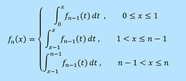
Below is the probability distribution for f5(x), where x is the sum of 5 real numbers from 0 to 1.
The distribution for f5 above is made of 5 smoothly joining degree 4 polynomial functions. The distribution for fn would be made of (n-1) smoothly joining degree (n-1) polynomial functions.
As n becomes very large, the chance of achieving a sum of 0 or n approaches zero. The width of 1 unit used in the recurrence integral becomes infinitely small relative to n, so the gradient of the function essentially depends on the value of the function itself, which results in an exponential function. But the gradient must be also be zero at the centre (the mean), and the function must be symmetrical about the mean. In fact, the gradient depends on both the height of the curve and the distance from the mean:
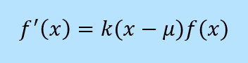
The solution to this differential equation gives the equation for the normal distribution, where μ is the mean and σ is the standard deviation.
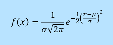
Below is a true normal distribution with a mean of 0 and a standard deviation of 1. It is remarkable how well the function f5 approximates the shape of the true normal distribution. It would be a hard task to pick the true normal curve if both of them were standing unlabelled in a police lineup!
Let's summarise what we have shown above:
- when we take several randomly chosen numbers, the sum is much more likely to be close to the middle than to the minimum or maximum
- if we have at least 3 numbers, the probability curve has a continuous gradient and the curve forms a bell shape
- if we have many numbers, the probability curve approaches a true normal distribution, which is defined by an exponential curve which is symmetrical about its mean
So you can see that when we take as few as 3-5 random numbers, the shape of the probability distribution for the sum already approaches the famous bell shape. And the same shape would apply to the average of the numbers, which is just the sum divided by how many there are.
So how does this relate to naturally occuring data such as height, weight etc? Well, let's take human height for example. Your height depends on many many causal factors. Most of these factors would be genetic, some may be environmental. These factors all contribute in some way to a weighted sum which determines your height. A normal distribution is still formed, even when the sum is "weighted" (i.e. some factors contribute more than others) and when the probability distribution for each factor is "skewed" (non-symmetrical). This is a consequence of the "central limit theorem" - check out this article for a simple explanation.
I hope this article has helped you to understand where the shape of the normal distribution comes from, and to further appreciate the beauty of the bell curve.
For a more rigorous derivation of the normal distribution formula, I recommend this paper by Saul Stahl. For a nice physical demonstration of the normal distribution in action, check out galtonboard.com